Today, we are going to look at how to compute and plot species accumulation curves (hereafter ‘SAC’) using the amazing vegan package. SAC’s are extremely popular in ecological analyses as they allow us to evaluate whether performing additional sampling is required to record all of the insect species associated with a particular plant species, for example.
In this session, we are going to cover the most basic SAC - observed richness. Observed species richness (hereafter ‘S’) simply tells us:
* how many species we have recorded, to date, and
* whether more surveys could yield new additional species.
* But, it DOES NOT tell us how many species could be in the community (i.e. we cannot extrapolate) - we will cover how to extrapolate species richness in a later post.
Let’s load in a typical community richness dataset (species abundance matrix). This dataset represents the insect community associated with the shurb, Lycium ferocissimum, in South Africa.
# Load required packages
if (!require("pacman")) install.packages("pacman")
pacman::p_load(tidyverse,
               tidyr,
               janitor,
               vegan)

# Read in data
sp_comm <- readr::read_csv("https://raw.githubusercontent.com/guysutton/CBC_coding_club/master/data_raw/species_abundance_matrix_ex.csv") %>%
  # Clean column names
  janitor::clean_names()

# Check data entry
dplyr::glimpse(sp_comm)
Rows: 56
Columns: 56
$ provinces                                   <chr> "Eastern Cape...
$ climatic_zones                              <chr> "Cfb", "Cfb",...
$ site                                        <chr> "EC1", "EC1",...
$ season                                      <dbl> 1, 2, 1, 2, 1...
$ haplotype                                   <dbl> 5, 5, 5, 5, 5...
$ cleta_eckloni                               <dbl> 23, 8, 11, 0,...
$ pseudambonea_capeni_schuhistes_lekkersingia <dbl> 4, 28, 0, 0, ...
$ acanthocoris_spinosus                       <dbl> 1, 0, 0, 0, 0...
$ antestiopsis_thunbergii                     <dbl> 1, 0, 0, 0, 0...
$ cassida_distinguenda                        <dbl> 0, 3, 0, 0, 0...
$ epilachna_sp_1                              <dbl> 0, 4, 0, 0, 0...
$ cleta_sp_1                                  <dbl> 0, 0, 0, 0, 0...
$ cleta_sp_2                                  <dbl> 0, 0, 0, 0, 0...
$ exochomus_flavipes                          <dbl> 0, 0, 0, 0, 0...
$ scymnus_sp                                  <dbl> 0, 0, 0, 0, 0...
$ cheilomenes_lunata                          <dbl> 0, 0, 0, 0, 0...
$ cheilomenes_sulphurea                       <dbl> 0, 0, 0, 0, 0...
$ cf_nephus_sp                                <dbl> 0, 0, 0, 0, 0...
$ chnootriba_sp                               <dbl> 0, 0, 0, 0, 0...
$ oenopia_cinctella                           <dbl> 0, 0, 0, 0, 0...
$ hippodamia_variegate                        <dbl> 0, 0, 0, 0, 0...
$ cassida_melanophthalma                      <dbl> 0, 0, 0, 0, 0...
$ cassida_reticulipennis                      <dbl> 0, 0, 0, 0, 0...
$ macetes_sp                                  <dbl> 0, 0, 0, 0, 0...
$ cryptocephalus_nr_liturellus                <dbl> 0, 0, 0, 0, 0...
$ epitrix_sp                                  <dbl> 0, 0, 0, 0, 0...
$ chrysomelidae_sp                            <dbl> 0, 0, 0, 0, 0...
$ sulcobruchus_longipennis                    <dbl> 0, 0, 0, 0, 0...
$ monolepta_bioculata                         <dbl> 0, 0, 0, 0, 0...
$ eurytomidae_sp                              <dbl> 0, 0, 0, 0, 0...
$ pachycnema_sp                               <dbl> 0, 0, 0, 0, 0...
$ scarabaeidae_sp                             <dbl> 0, 0, 0, 0, 0...
$ neoplatygaster_serieturberculata            <dbl> 0, 8, 0, 0, 0...
$ sciobius_sp                                 <dbl> 0, 0, 0, 0, 0...
$ lixini_sp                                   <dbl> 0, 0, 0, 0, 0...
$ beaufortiana_cornuta                        <dbl> 0, 0, 0, 0, 1...
$ pentatomidae_sp                             <dbl> 0, 0, 0, 0, 0...
$ apalochrus_sp                               <dbl> 0, 0, 0, 0, 0...
$ hylomela_sexpunctata                        <dbl> 0, 0, 0, 0, 1...
$ anthripidae_sp                              <dbl> 0, 0, 0, 0, 1...
$ cenaeus_carnifex                            <dbl> 0, 0, 0, 0, 0...
$ thrips_simplex                              <dbl> 0, 0, 0, 0, 0...
$ ceratitis_sp                                <dbl> 0, 0, 0, 0, 0...
$ brachymeria_sp                              <dbl> 0, 0, 0, 0, 0...
$ syrphidae_sp                                <dbl> 0, 0, 0, 0, 0...
$ cicadidae_sp                                <dbl> 0, 0, 0, 0, 0...
$ apis_mellifera                              <dbl> 0, 0, 0, 0, 0...
$ pteromalidae_sp                             <dbl> 0, 0, 0, 0, 0...
$ chrysopidae_sp                              <dbl> 0, 0, 0, 0, 0...
$ pamphagidae_sp                              <dbl> 0, 0, 0, 0, 0...
$ amphipsocidae_sp                            <dbl> 0, 0, 0, 0, 0...
$ diptera_sp                                  <dbl> 0, 0, 0, 0, 0...
$ hymenoptera_sp                              <dbl> 0, 0, 0, 0, 0...
$ decapotoma_lunata                           <dbl> 0, 0, 0, 0, 0...
$ pyrrhocordae_sp_1                           <dbl> 0, 0, 0, 0, 0...
$ mylabris_oculata                            <dbl> 0, 0, 0, 0, 0...
Now it is time to compute our species accumulation curve. To do this, we will use the poolaccum function from the vegan R package. Notice the first few columns are site description variables (i.e. not species abundances). We need to remove these columns, and only input the columns containing species abundances.
We now need to extract our observed species richness (S) estimates.
- N - No. of surveys (i.e. survey effort)
- S - Observed species richness
- lower2.5 - lower 95% confidence interval of S
- upper97.5 - upper 95% confidence interval of S
# Extract observed richness (S) estimate
obs <- data.frame(summary(sac_raw)$S, check.names = FALSE)
colnames(obs) <- c("N", "S", "lower2.5", "higher97.5", "std")
head(obs)
N S lower2.5 higher97.5 std
1 3 7.17 0.000 15.000 3.787419
2 4 9.13 2.000 18.000 4.222726
3 5 10.87 2.475 18.525 4.464574
4 6 12.49 4.475 21.525 4.641697
5 7 14.38 6.000 22.525 4.442176
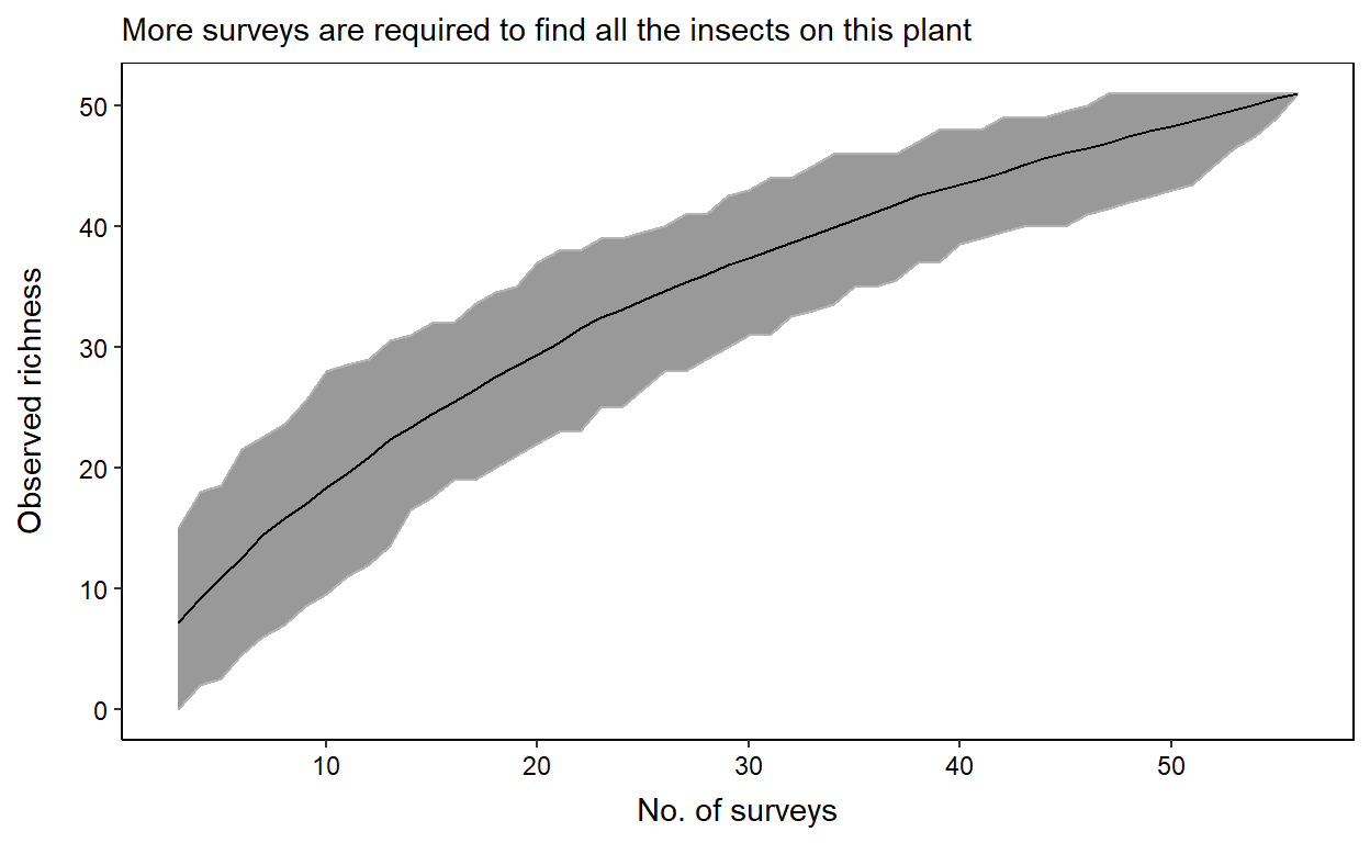
6 8 15.81 7.000 23.575 4.622508Finally, we can plot the desired species accumulation curve. Ultimately, we would like to see our S estimate and the 95% confidence intervals reach an asymptote (flat line) on the y-axis. This would indicate that performing additional surveys is highly unlikely to yield additional insects on the plant we have surveyed.
obs %>%
  ggplot(data = ., aes(x = N,
                       y = S)) +
  # Add confidence intervals
  geom_ribbon(aes(ymin = lower2.5,
                  ymax = higher97.5),
              alpha = 0.5,
              colour = "gray70") +
  # Add observed richness line
  geom_line() +
  labs(x = "No. of surveys",
       y = "Observed richness",
       subtitle = "More surveys are required to find all the insects on this plant")